Tutorial 2
Installation of SNAP and NetworkX
Recomended: Anaconda Scientific Python Distribution is the preferred and easiest way to enjoy python and its applications on data analysis, including social network data analysis, using python packages like SNAP and NetworkX. Anaconda already integrate most popular Python packages for science, math, engineering, data analysis, including NetworkX, so it saves you a lot of time figuring out all the dependency of python packages and installing them one by one in order.
- Installation steps:
- Download Anaconda, select the correct version corresponds to your OS by clicking the icons after CHOOSE YOUR INSTALLER, there are also installation tips in each OS version shower in the window.
- After the installation of Anaconda, you already have Python, Ipython, Ipython Notebook, NetworkX, which are the things we will use in this course.
- Suppose you installation path of Anaconda is "AnacondaPath", inside "AnacondaPath/bin/" folder there are commands like python, ipython, you can enter python either by clicking them or by running "AnacondaPath/bin/python" in your terminal, also you should be able to import networkx package. For example, in my computer(Linux),
[rzheng@SymLab ~]$ ./workspace/anaconda-2.1.0/bin/python
Python 2.7.8 |Anaconda 2.1.0 (64-bit)| (default, Aug 21 2014, 18:22:21)
[GCC 4.4.7 20120313 (Red Hat 4.4.7-1)] on linux2
Type "help", "copyright", "credits" or "license" for more information.
Anaconda is brought to you by Continuum Analytics.
Please check out: http://continuum.io/thanks and https://binstar.org
>>> import networkx
>>>
- Ipython Notebook is highly recommended for the purpose of education and self-learning, it enables an interactive experience of using python, and it uses web browser for the rendering of all the intermediate steps including your code snippets and results so you can share your notebooks/experiences with others. For example, in my computer, firefox (my default web browser) will be opened and i can create new notebook and run python codes based on the browser after running the following bash commands.
[rzheng@SymLab tmp]$ ~/workspace/anaconda-2.1.0/bin/ipython notebook
2015-02-08 17:24:39.561 [NotebookApp] Using existing profile dir: u'/home/rzheng/.ipython/profile_default'
2015-02-08 17:24:39.570 [NotebookApp] Using MathJax from CDN: https://cdn.mathjax.org/mathjax/latest/MathJax.js
2015-02-08 17:24:39.612 [NotebookApp] Serving notebooks from local directory: /home/rzheng/tmp
2015-02-08 17:24:39.613 [NotebookApp] 0 active kernels
2015-02-08 17:24:39.613 [NotebookApp] The IPython Notebook is running at: http://localhost:8888/
2015-02-08 17:24:39.613 [NotebookApp] Use Control-C to stop this server and shut down all kernels (twice to skip confirmation).
- SNAP is not included in Anaconda, so we have to install its python bindings by ourselves, but it's easy. Download the right version for your OS, unzip it, and then install it using the python inside Anaconda, instead of the python integrated by your OS. For example, in linux,
[rzheng@SymLab workspace]$wget http://snap.stanford.edu/snappy/release/snap-1.1-2.3-centos6.5-x64-py2.6.tar.gz
[rzheng@SymLab workspace]$ tar zxvf snap-1.1-2.3-centos6.5-x64-py2.6.tar.gz
[rzheng@SymLab workspace]$cd snap-1.1-2.3-centos6.5-x64-py2.6
[rzheng@SymLab snap-1.1-2.3-centos6.5-x64-py2.6]$ ~/workspace/anaconda-2.1.0/bin/python setup.py install
[rzheng@SymLab snap-1.1-2.3-centos6.5-x64-py2.6]$ ~/workspace/anaconda-2.1.0/bin/python
Python 2.7.8 |Anaconda 2.1.0 (64-bit)| (default, Aug 21 2014, 18:22:21)
[GCC 4.4.7 20120313 (Red Hat 4.4.7-1)] on linux2
Type "help", "copyright", "credits" or "license" for more information.
Anaconda is brought to you by Continuum Analytics.
Please check out: http://continuum.io/thanks and https://binstar.org
>>> import networkx
>>> import snap
>>>
# Simple example
import networkx as nx     # nx can be seemed as an alias of networkx module
G = nx.Graph()            # create an empty graph with no nodes and no edges
print G.nodes(), G.edges()
G.add_node(1)    # add a single node
print G.nodes()
G.add_nodes_from([2,3])    # add a list of nodes
print G.nodes()
G.clear(); G.add_node(1)    # clear the graph and add a node
H = nx.path_graph(10)  # generate a bunch of nodes
print H
G.add_nodes_from(H)    # add all the nodes in H, repeated nodes "1" will not be added again
print G.nodes()
G.add_node(H)          # add H as a node of the graph
print G.nodes()
G.add_edge(1,2)
print G.nodes(), G.edges()
e=(2,3)
G.add_edge(*e) # unpack edge tuple
print G.edges()
G.remove_edges_from(G.edges())  # clear edges
print G.edges()
G.add_edges_from([(1,2), (1,3)]) # add edges from a edge list
print G.edges()
G.add_node("spam")  # add one node called "spam"
G.add_nodes_from("spam") # add 4 nodes: 's', 'p', 'a', 'm', since string "spam" in python is actually a list ['s', 'p', 'a', 'm']
print G.nodes(), G.number_of_nodes()
G.neighbors(1) # neighbor of node 1
G.remove_nodes_from("spam")  # remove a list of nodes
print G.nodes()
G.remove_edge(1,3)  # remove an edge
print G.edges()
H = nx.DiGraph(G)    # create a DiGraph using the connections from G
print H.nodes(), H.edges()
edgelist = [(0,1), (1,2), (2,3)]
H = nx.Graph(edgelist)    # create a graph using edgelist
print H.nodes(), H.edges()
print G[1]    # node 1's attributes, including neighbors and edge attributes
G.add_edge(1,3)
G[1][3]['color'] = 'blue'
print G[1]
# fast examination of all edges using adjacency iterators
FG = nx.Graph()
FG.add_weighted_edges_from([(1,2,0.125), (1,3,0.75), (2,4,1.2), (3,4,0.375)])    # add weighted edges
for n, nbrs in FG.adjacency_iter():  # n: node, nbrs: corresponding neighbors
    for nbr, edge_attr in nbrs.items():
        data = edge_attr['weight']
        print '(%d, %d, %.3f)' % (n, nbr, data)
G = nx.Graph(day='Friday')  # graph has an attribute day which is set to be Friday
print G.graph, G.nodes(), G.edges()
G.graph['day'] = 'Monday'  # modify the attribute
print G.graph
G.add_node(1, time = '5pm')
G.add_nodes_from([3, 4], time = '2pm')
print G.node[1]
G.node[1]['room'] = 123
print G.nodes(),'\n', G.nodes(data=True)
G.add_edge(1, 2, weight=4.7)
G.add_edges_from([(3,4), (4,5)], color='red')
G.add_edges_from([(1,2,{'color':'blue'}), (2,3,{'weight':8})])
print G.edges(data=True)
G.edge[1][2]['weight'] = 4 # or G[1][2]['weight'] = 4
print G.nodes(data=True), '\n', G.edges(data=True)
DG = nx.DiGraph()
DG.add_weighted_edges_from([(1,2,0.5), (3,1,0.75)])
print DG.in_degree(1, weight = 'weight'), DG.out_degree(1, weight = 'weight'), DG.degree(1, weight = 'weight')
print DG.in_degree(1), DG.out_degree(1), DG.degree(1)
print DG.successors(1), DG.predecessors(1), DG.neighbors(1) # neighbors in directed graph are equivalent to successors
# H = nx.Graph(G) # conver to undirected graph
MG = nx.MultiGraph()    # multigraph allow multiple edges between an pair of nodes
MG.add_weighted_edges_from([(1,2,.5), (1,2,.75), (2,3,.5)])    # allow to add the same edge twice, possibly with different edge data
print MG.degree(weight = 'weight'), '\n', MG.edges(data = True)
# many algorithms are not well defined in multigraph (shortest path .e.g), in such cases should convert to standard graph
GG = nx.Graph()
for n, nbrs in MG.adjacency_iter():
    for nbr, edata in nbrs.items():
        minvalue = min([d['weight'] for d in edata.values()]) # find the minimum weight edge between n-nbr
        GG.add_edge(n, nbr, weight = minvalue)                # add a single edge between n-nbr with minimum weight

print GG.edges(data=True), '\n', nx.shortest_path(GG, 1, 3)
G = nx.Graph()
G.add_edges_from([(1,2), (1,3)])
G.add_node("spam")
print nx.connected_components(G), '\n', sorted(nx.degree(G).values()), '\n', nx.degree(G)
print nx.degree(G, [1,2]), G.degree([1,2]), sorted(G.degree([1,2]).values())  # nx.degree(G, nodelist) is equal to G.degree(nodelist)
print nx.clustering(G)  # compute the clustering coefficients of G
G.add_edge(2,3)
print nx.clustering(G)
import matplotlib.pyplot as plt
%matplotlib inline
plt.figure(figsize=(6,4))
nx.draw(G)
plt.show()
# plt.savefig("path.png")
NetworkX+d3.js for better visualization, example from IPython Cookbook by Cyrille Rossant
Tutorial 4
Network Must-Known Concepts
- Undirected / Directed, Connected / Disconnected, Weighted / Unweighted
- Strongly Connected vs Directed Acyclic Graph
- Strongly Connected: Any node can reach any other node via a directed path
- Any directed graph \(G(V,E)\) can be seemed as a directed acyclic graph \(G^{'}(V^{'},E^{'})\) with \(V^{'}\) are the strongly connected components of \(G(V,E)\)
import networkx as nx
import numpy as np
import matplotlib.pyplot as plt
import pylab
%matplotlib inline
G = nx.DiGraph()
G.add_edges_from([('A','B'),('B','C'),('C','D'),('D','B'),('E','D')])

plt.figure(figsize=(3,2))
nx.draw(G, pos=nx.circular_layout(G), node_size=500)  # layout: positioning algorithms for graph drawing, here use circular_layout,
plt.show()                                            # "arrows" for directed graph are drawn with just thicker stubs by default
print nx.strongly_connected_components(G), '\n', nx.weakly_connected_components(G), '\n', nx.is_strongly_connected(G)

# draw all the strongly connected components
#for _ in nx.strongly_connected_component_subgraphs(G):
#    plt.figure(figsize=(2,1))
#    nx.draw(_)
Adjacency Matrix, Sparse Graph, Complete Graph
A cool visualization of Adjacency Matrix, select order by cluster and compare the matrix with Another cool visualization of Network, see if you can find the corresponding group in the network for each block in the matrix, both visualization use d3.js library and Les Miserables dataset.
A = nx.adjacency_matrix(G)  # adjacency_matrix returns a sparse matrix, can be converted to dense matrix by A.todense() method
print G.nodes(), '\n\n', A, '\n\n'

# convert to undirected graph
print nx.adjacency_matrix(G.to_undirected())
- Degree Distribution, Clustering Coefficient, Distance
# generate a random graph
G = nx.random_graphs.fast_gnp_random_graph(200, 0.03) # n: 200, p: 0.03, expected degree will be (n-1)p
pos = nx.spring_layout(G)
plt.figure(figsize=(8,6))
nx.draw_networkx_nodes(G, pos, node_size=20, with_labels=False)
nx.draw_networkx_edges(G, pos, alpha=0.4)
plt.axis('off')
plt.show()
# import bokeh package for nice and interactive plot
from bokeh.charts import Histogram
from bokeh.plotting import *
output_notebook()
degree_sequence = sorted(nx.degree(G).values(), reverse=True)

p1 = figure(title="Degrees", width=500, height=350)
p1.circle(range(len(degree_sequence)), degree_sequence, color="red")
p1.xaxis.axis_label = 'Node (after sorted)'
p1.yaxis.axis_label = 'Degree'

bins = np.arange(min(degree_sequence)-0.5, max(degree_sequence)+1, 1)

# using bokeh high-level charts interface
#hist = Histogram(degree_sequence, bins=max(degree_sequence)-1, ylabel="frequency",
#                 xlabel="degree", width=500, height=350, notebook=True)
#hist.show()

# using simple bokeh plot function
h, bins = np.histogram(degree_sequence, density=True, bins=bins)
#print degree_sequence,'\n',h,'\n',bins
p2 = figure(title="Degree Distribution", width=500, height=350)
p2.quad(top=h/sum(h), bottom=0, left=bins[:-1]+0.03, right=bins[1:]-0.03, alpha=0.6, fill_color="red", line_color="red")
p2.xaxis.axis_label = 'Degree'
p2.yaxis.axis_label = 'Frequency'
show(VBox(p1,p2))
clustering_sequence = sorted(nx.clustering(G).values(), reverse=True)
p1 = figure(title="Clustering Coefficients", width=500, height=350)
p1.circle(range(len(clustering_sequence)), clustering_sequence, color="green")
p1.xaxis.axis_label = 'Node (after sorted)'
p1.yaxis.axis_label = 'Clustering Coefficient'

p2 = figure(title="Clustering Coefficient Distribution", width=500, height=350)
bins = np.arange(min(clustering_sequence), max(clustering_sequence), 0.02)
h, bins = np.histogram(clustering_sequence, density=True, bins=bins)
#print h, bins, sum(h)
p2 = figure(title="Clustering Coefficient Distribution", width=500, height=350)
p2.quad(top=h/sum(h), bottom=0, left=bins[:-1]+0.0008, right=bins[1:]-0.0008, alpha=0.6, fill_color="red", line_color="red")
p2.xaxis.axis_label = 'Clustering Coefficient'
p2.yaxis.axis_label = 'Frequency'

show(VBox(p1,p2))
- Centrality Measures
- Node centrality: How central/important/influential each node is?
- Degree Centrality: total number of neighbors
- Betweenness Centrality / Katz Centrality: total number of shortest paths / paths that goes through
- Closeness Centrality: 1/(total length of distances to all the other nodes)
- Eigenvector Centrality: total centrality of neighbors + centrality should be self consistant / balanced, \(A\mathbf{x} = \lambda \mathbf{x}\). Algorithm Understanding: suppose \(\mathbf{v}_i\) is \(i\)th eigenvector of \(A\), and \(\mathbf{v}_i^{max}\) is the eigenvector with maximum absolute eigenvalue (mathematically called spectral radius), \(\mathbf{x} = \sum_{i}c_i\mathbf{v}_i\) is the expansion of \(\mathbf{x}\) in the eigenspace of \(A\), so \(A^k\mathbf{x} = \sum_{i}c_i\lambda_i^{k}\mathbf{v}_i\), then for any vector \(\mathbf{x}\) that is not orthogonal with \(\mathbf{v}_i^{max}\), which means \(c_i^{max} \neq 0\), \(A^k\) act on \(\mathbf{x}\) is equal to first project \(\mathbf{x}\) into eigenspace of \(A\), then keep rescaling each component \(c_i\lambda_i^{k-1}\mathbf{v}_i\) by corresponding eigenvalue \(\lambda_i\), when \(k\to \infty\), the component in \(\mathbf{v}_i^{max}\) direction will dominate. Normalization step is to avoid blowing up from \(\lambda_i^k\). But why we choose the eigenvector with maximum eigenvalue as the centrality measure instead of any eigenvector? 1, Assumption of each element in \(\mathbf{x}\) should be \(\gt 0\); 2, Perron–Frobenius theorem.
- Normalization: total number -> total number / maximum total number, total length -> total length / minimum total length
- Network centralization: How central the most central node is in relation to how central all the other nodes are? An extension can be how much variation/heterogeneity the network has? Every node centrality measure has a corresponding centralization measure.
Network Models
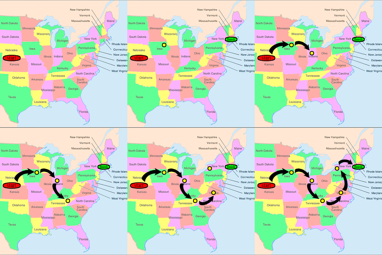
- Small World: average path length for social networks, 6-degree.
Stanley Milgram's Experiment:
- Model Comparison:
| ER Model | WS Model | BA Model | |
|---|---|---|---|
| Description | \(G(N,p)\): Given \(N\) nodes, each pair is linked with probability \(p\) | \(G(N,K,p)\): Start from a regular ring lattice with \(N\) nodes, and each node is connected with its \(K\) nearest neighbors, with probability \(p\) replace each lattice edge with a new random edge | \(G(N, m, m_0)\), Start from an intial connected network of \(m_0\) nodes, each new added node is connected to \(m\) existing nodes (\(m\lt m_0\)) in a preferential attachment way |
| \(P(k)\): degree distribution | Binomial: \(B(k;N-1,p)\xrightarrow{N\to\infty,Np\equiv \lambda}\) Poisson: \(P(k;\lambda)\) | Dirac delta function: \(\delta_{k,K}\xrightarrow{p\to 1}\) ER Model, the shape of the degree distribution is similar to ER Model and has a pronounced peak at \(k=K\) and decays exponentionally for large \(|k-K|\) | \(\sim k^{-3}\) when \(N\to\infty\) |
| \(\overline k\): average degree | \((N-1)p\) | relatively homogeneous, all nodes have more or less the same degree, peaked at \(K\) | divergent when \(N\to\infty\) |
| \(\overline C\): average clustering coefficient | \(p\) usually a tiny value, think of how many friends you could have in your life and 7 billion people there | High: \(\frac{3}{4} \xrightarrow{p\to 1}\) Low: \(\frac{K}{N}\) | Significantly higher, \(\sim N^{-0.75}\) |
| \(\overline l\): average path length | Short: \(\frac{\ln N}{\ln\overline k}\), \(\mathcal{O}(\log N)\) | Long: \(\frac{N}{2K}\), \(\mathcal{O}(N) \xrightarrow{p\to 1}\) Short: \(\frac{\ln N}{\ln K}\), \(\mathcal{O}(\log N)\) | \(\sim \frac{\ln N}{\ln\ln N}\), even shorter than ER model |
| Scale free? | NO | NO | Yes, both growth and preferential attachment are needed |
| Advantage/Disadvantage | A: simple D: 1, don't generate local custering and triadic closures, therefore low clustering coefficient; 2, no formation of hubs, not scale free |
A: Address the first limitation of ER model, accounts for clustering while retaining the short average path length of ER model D: 1, a fixed number of nodes thus cannot be used to model network growth; 2, unrealistic degree distribution |
A: incorporates two important concepts: network growth and preferential attachment D: clustering is not independent of system size |
Visualization of Networks
Tutorial 5
Concepts Clarification
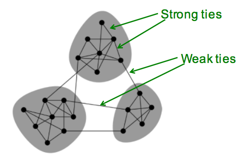
Granovette's theory
- Weak tie (socially weak, but structually important for information flow) \(\leftarrow\) Strength \(\to\) Strong tie (socially strong, but heavily redundant in terms of information access)
- Bridge: if removed leads to disconnected graph; Local Bridge: edges of span \(\gt 2\), span is the distance of the edge endpoints if the edge is deleted
- Tradic Closure: two strong ties \(A-B\), \(A-C\), imply a third edge \(B-C\) (can be either strong or weak)
Local Bridges and Weak Ties:
The reason why \(A\) should be involved in at least \(2\) strong ties is because if \(A\) only has one strong tie, that strong tie itself could be a local bridge and it does not violate tradic closure assumption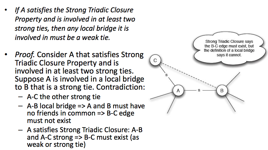
- Edge Overlap: \(O_{ij} = \frac{N(i)\bigcap N(j)}{N(i)\bigcup N(j)}\), where \(N(i)\) are the neighbors of node \(i\) (not include \(j\)), the endpoints of a local bridge have no common neighbor, therefore overlap is 0
- In cell-phone network, highly used (strong) links has high overlap (strong locality)
Keep this picture in mind:
Burt's theory
- Structural Hole: To understand what does it mean
Understand the importance of bridging role / middleman / broker.
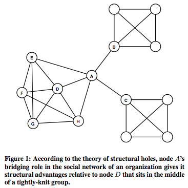
Information within clusters tends to be rather homogeneous and redundant. Non-redundant information is most often obtained through contacts in different clusters. When two separate clusters possess non-redundant information, there is said to be a structural hole between them. Structural hole is lack of connection between two nodes that is bridged by a broker.
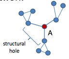
Since individuals can benefit from serving as intermediaries between others who are not directly connected, this leads to Strategic Network Formation which studies the evolution of network when individuals in a social network have incentives to form links that bridge otherwise disconnected parties. Check the following talk, if you only want to know what is structural hole, check the first 15 minutes; if you are interested in applying game theoretical model on strategic network formation problem, check the full video
from IPython.display import YouTubeVideo

YouTubeVideo('yEY9_HwvnqU')
Network Constraint: It is one metric to find bridgers (other metrics can be betweenness centrality .e.g). An individual's network constraint measures the extent to which he links to others that are already linked to each other. Low network constraint means that an individual has links to others who are not already linked to each other. High betweenness centrality and low network constraint both indicate bridging. How to calculate network constraint? \[p_{ij} = \frac{w_{ij}}{\sum_{j\in N(i)}{w_{ij}}}\] \(w_{ij}\) is the weight of edge \(e_{ij}\) (.e.g 1 for strong tie, 0.5 for weak tie), \(p_{ij}\) indicates how much time/energy \(i\) spends on \(j\), with this definition of \(p_{ij}\), the network constraint of \(i\) is defined as \[C_i = \sum_{j\in N(i)}{c_{ij}} = \sum_{j\in N(i)}[p_{ij} + \sum_{k\in N(i)}(p_{ik}p_{kj})]^2\]
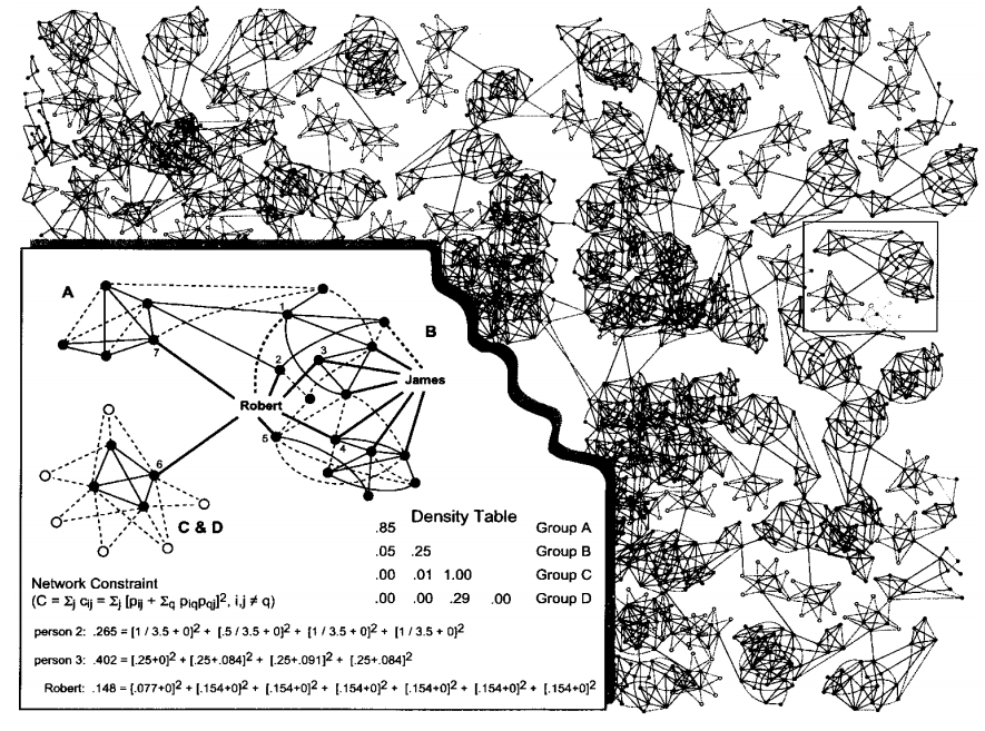
In the above picture, for person 2 and Robert, there is no links among their neightbors, for person 3, there is triangulars among him and his neighbors. So low constraint \(\Rightarrow\) contacts are disconnected, high constraint \(\Rightarrow\) contacts are close
Community Detection
- Betweenness
- Definition: node/edge betweenness is the number of shortest paths between pairs of nodes that path through the node/edge
Algorithm for calculation of betweenness (Brandes' algorithm, for unweighted graph ):
\(d[w]\) is the distance to the root node \(s\), \(P[w]\) saves the parent nodes of node \(w\), \(\sigma[w]\) is the number of shortest paths from root node \(s\) to node \(w\); \(\delta[w]\) is used to accumulates the weighted flow from its children nodes and also distributes it to its parent nodes(.e.g \(v\)) with weight \(\sigma[v] / \sigma[w]\); \(C_B\) is the node betweenness centrality.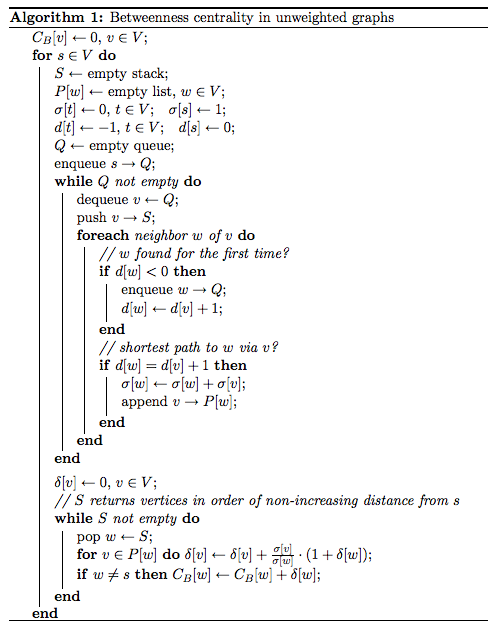
- Girvan-Newman algorithm: progressively removing edges from the original network \(\to\) dendrogram
Modularity
- Definition: from Wiki: Modularity: one measure of the structure of networks or graphs, measure the strength of division of a network into modules (also called groups, clusters or communities). Networks with high modularity have dense connections between the nodes within modules but sparse connections between nodes in different modules.
- How to turn a given graph (.e.g in total \(n\) nodes where each node \(i\) has degree \(k_i\), and \(m\) edges) into a random graph and still keep the degree of each node unchanged? Concept of configuration models is a randomized realization of a particular network: cuts each edge into two halves, and then each half edge, called a stub, is rewired randomly with any other stub in the network even allowing self loops (multigraph). In this way, the total number of stubs is \(\sum_{i}k_i = 2m\), the probability of choosing any stub from node \(j\) is \(\frac{k_j}{2m}\), the expected number of edges between \(i\) and \(j\) in the completely random graph will be \(\frac{k_ik_j}{2m}\)
- For a Graph \(G\), define modularity \(Q(G,S)\) with respect to a community partition \(S\) as \[Q(G,S) = \frac{1}{2m} \sum_{s\in S}\sum_{i,j\in s}[A_{ij}-\frac{k_ik_j}{2m}] = \sum_{i,j}[\frac{A_{ij}}{2m} - \frac{k_ik_j}{4m^2}]\delta(c_i,c_j)\] \(A\) is adjacency matrix, \(c_i\) is the community index which \(i\) belongs to in partition \(S\), \(\delta(c_i,c_j) = 1\) when \(c_i = c_j\), otherwise 0
- Modularity Matrix formulation: define \(Z_{ir}\) to be 1 if \(c_i = r\) and zero otherwise, then \(Z\) is a \(n \times |S|\) matrix (membership matrix, each row \(Z_{i\bullet}\) is a length \(|S|\) membership vector for node \(i\)), so \[\delta(c_i, c_j) = \sum_rZ_{ir}Z_{jr}\] \[Q(G,S) = \frac{1}{2m} \sum_{i,j}\sum_{r} [A_{ij} - \frac{k_ik_j}{2m}]Z_{ir}Z_{jr} = \frac{1}{2m}Tr(Z^TBZ)\] \(B\) is called modularity matrix with \(B_{ij} = A_{ij} - \frac{k_ik_j}{2m}\)
- Goal: maximize modularity, with this goal come with different community detection algorithms, for those who are interested check this slides
Practical Skills
Gephi
NetLogo
Be sure to check the Syllabus of Lada Adamic's course @ coursera, there are many netlogo models provided there for you to play with, don't miss the funny part of this course.
Tutorial 6
This notebook is adapted by TA YiuFung Cheong from CH1 of this wonderful book: Mining the Social Web 2nd Edition
Lab 6 Mining Twitter using API
In this lab we will learn how to use Twitter API to retrieve information that you are interested in. For example, we will explore trending topics, what other users are talking about, and more.
Full code is available in GitHub.
This tutorial is an adaptation of Chapter 1 from the book Mining the Social Web, 2nd Edition which uses Simplified BSD License. We thank the original authors for their contribution.
Installation
Twitter has taken great care to craft an elegantly simple RESTful API that is intuitive and easy to use. Even so, there are great libraries available to further mitigate the work involved in making API requests. A particularly beautiful Python package that wraps the Twitter API and mimics the public API semantics almost one-to-one is twitter.
In this tutorial, we will use twitter to make API calls. This is a python wrapper for twitter APIs.
For Mac and Linux students, you can install this package in a terminal with pip with the command pip install twitter, preferably from within a Python virtual environment.
For Windows students, please run
Scripts\pip.exe install twitterunder Anaconda installation directory, that is C:\Users\your_name\Anaconda.
# Run this cell to make sure you install
import twitter # There should be no error.
Authentication
Now we are ready to play with Twitter API. Before that, we will talk about OAuth.
Suppose you just develop a game based on twitter and would like to share with your friends. To retrieve twitter-related information, you may just input your username and password to access the API. This might work fine for you, but your friend or colleague probably wouldn’t feel comfortable inputing plain text username and password in your application. After all, who knows whether your application is doing something strange behind? Even you are trusted by them, it's never a good idea to store password in plain text as once your application is cracked they will be all leaked. Therefore, we need a way for authorization without giving up our credentials.
OAuth is designed to cope with these situations. OAuth stands for "Open Authorization". It specifies a process for resource owners (your friend) to authorize third-party (your application) access to their server resources (twitter user name, bio, following etc.) without sharing their credentials. Designed specifically to work with Hypertext Transfer Protocol (HTTP), OAuth essentially allows access tokens to be issued to third-party clients by an authorization server, with the approval of the resource owner.
Some useful terms:
1. Third Party Applications: or `client`. For example, your game.
2. HTTP Service: or simply service. For example, twitter.
3. Resource owner: the user of your application.
4. Authorization server: the server of HTTP service that's in charge of authorization.
5. Resource server: the server of HTTP service that stores user information.
Note that authorization server and resource server can be the same machine, or not, or a distributed data farm.
The protocol flow of OAuth is demonstrated in RFC 6749
 +--------+                               +---------------+
 |        |--(A)- Authorization Request ->|   Resource    |
 |        |                               |     Owner     |
 |        |<-(B)-- Authorization Grant ---|               |
 |        |                               +---------------+
 |        |
 |        |                               +---------------+
 |        |--(C)-- Authorization Grant -->| Authorization |
 | Client |                               |     Server    |
 |        |<-(D)----- Access Token -------|               |
 |        |                               +---------------+
 |        |
 |        |                               +---------------+
 |        |--(E)----- Access Token ------>|    Resource   |
 |        |                               |     Server    |
 |        |<-(F)--- Protected Resource ---|               |
 +--------+                               +---------------+
So the steps are:
The client requests authorization from the resource owner.
The client receives an authorization grant, which is a credential representing the resource owner's authorization.
The client requests an access token by authenticating with the authorization server and presenting the authorization grant.
The authorization server authenticates the client and validates the authorization grant, and if valid, issues an access token.
The client requests the protected resource from the resource server and authenticates by presenting the access token.
The resource server validates the access token, and if valid, serves the request.
Nowadays, many applications use OAuth. See a list here. Understanding OAuth will help with data collection when using APIs on websites such as Facebook, Fitbit, Flickr, Instagram etc.
Playing with Twitter APIs
Before you can make any API requests to Twitter, you’ll need to create an application at https://apps.twitter.com/. If you don't have a twitter account, register one and it's fun :)
Steps to create an application:
1. Press Create New App and follow the steps.

2. In `Keys and Access Tokens`, press `Create My Access Token`:
    This step let you authrorize your own application to access your account info.

3. Copy paste related values into the next cell and run it. If everything goes well, now you have a new twitter_api handle.
    Be careful when copy paste the keys and secrets and make sure no spaces are added.

4. Go to your twitter page and follow a few accounts from the recommendation. We will test our API using them.
Note that Twitter has its API Rate Limits. API Rate Limit is counted in a 15-min time window. Inside this time window, you cannot make more than a specified number of requests, or else you will get rate exceeded error. For example, no more than 15 requests for followers/id in this window for application authorization mode. Different API will have different rate limits, for example, you can have 180 requests for your timeline in this time window.
So do not refresh too frequently or you will need to wait a while. This will also impose some restriction on your data collection process.
Example 1. Authorizing an application to access Twitter account data
import twitter
import json # to prettify output

# XXX: Go to http://dev.twitter.com/apps/new to create an app and get values
# for these credentials, which you'll need to provide in place of these
# empty string values that are defined as placeholders.
# See https://dev.twitter.com/docs/auth/oauth for more information
# on Twitter's OAuth implementation.

CONSUMER_KEY = ''
CONSUMER_SECRET =''
OAUTH_TOKEN = ''
OAUTH_TOKEN_SECRET = ''

auth = twitter.oauth.OAuth(OAUTH_TOKEN, OAUTH_TOKEN_SECRET,
                           CONSUMER_KEY, CONSUMER_SECRET)

t = twitter.Twitter(auth=auth)

# Nothing to see by displaying t except that it's now a
# defined variable

print t
Example 2. Some basic usages.
twitter package simply wraps official RESTful API into a python class. You access the members as decoded python objects (lists and dicts).
# Timeline related.

# Get your "home" timeline and print the text of first one.
my_timeline = t.statuses.home_timeline()
for tweet in my_timeline:
    print tweet['text']

print "=================================================================="

# Get a particular user's timeline
tl_9Gag = t.statuses.user_timeline(screen_name="9GAG")
for tweet in tl_9Gag:
    print tweet['text']

print "=================================================================="

# to pass in GET/POST parameters, such as `count`
# this means retrieve the most recent 5 tweets (default 20, max 200) on your own timeline.
# see https://dev.twitter.com/rest/reference/get/statuses/home_timeline
print t.statuses.home_timeline(count=5)[4]['text']
# Relationships related API.

# We will take the great scientist Richard Dawkins as an exmample.
# https://twitter.com/RichardDawkins

# Some commonly seen terms:
# screen_name: the name after @
# id: the id corresponds to the user. Note that id is static, while screen_name can be changed by the user.
# friends: people the specified user follows.
# followers: people who follows the specified user

# So, Richard Dawkins' screen_name is "RichardDawkins" (no space). He has 305 friends and 1.14M followers.

# Now try to get the data using API.

# Get all his followings, or "friends" in Twitter's context.
# See https://dev.twitter.com/rest/reference/get/friends/ids
friends = t.friends.ids(screen_name="RichardDawkins")
print friends['ids']

# Get all his followers
# See https://dev.twitter.com/rest/reference/get/followers/ids
followers = t.followers.ids(screen_name="RichardDawkins")
print followers['ids']
# But all you get is just id.
# We need to transform an id to a real user object.

# Transform multiple user_id to a list of user objects
# See https://dev.twitter.com/rest/reference/get/users/lookup
# Note that this API transform at most 100 user_id at one time, so we pass the first 100 users.
# Or else, an error will be returned by twitter.
friends_profile = t.users.lookup(user_id=friends['ids'][:100])
print friends_profile[0]['screen_name'] # print the first one.
print "================================================================"
print json.dumps(friends_profile, indent=1)
# You can also use users/show to transform a single user_id to a user object
# See https://dev.twitter.com/rest/reference/get/users/show
print json.dumps(t.users.show(screen_name="RichardDawkins"), indent=1)
# Let's go back to check friends and followers result.

print "friend count is", len(friends['ids'])
print "followers count is", len(followers['ids'])
# You can see that number of followers is WRONG!
# Richard Dawkins has 1.14M followers.
# It's too large for Twitter to return the response to you all at once.

# Twitter uses a mechanism called "cursoring" to paginite large results.
# Results are returned in a batch. In this case, followers ids are returned in a batch of 5000.
# To get the next batch, we will use the next_cursor in the next API request.
# See https://dev.twitter.com/overview/api/cursoring
print followers['next_cursor']

# Get the next batch using next_cursor as argument.
next_batch = t.followers.ids(screen_name="RichardDawkins", next_cursor=followers['next_cursor'])
print next_batch

# Note that you can get the previous batch using previous_cursor.
Example 3. Collecting Search Results
Let's see how people feels about Apple Event last week.
# Import unquote to prevent url encoding errors in next_results
from urllib import unquote

# XXX: Set this variable to a trending topic,
# or anything else for that matter. The example query below
# was a trending topic when this content was being developed
# and is used throughout the remainder of this chapter.

q = '#AppleEvent'

count = 100

# See https://dev.twitter.com/docs/api/1.1/get/search/tweets

search_results = t.search.tweets(q=q, count=count)

statuses = search_results['statuses']

# Iterate through 5 more batches of results by following the cursor

for _ in range(5):
    print "Length of statuses", len(statuses)
    try:
        next_results = search_results['search_metadata']['next_results']
    except KeyError, e: # No more results when next_results doesn't exist
        break

    # Create a dictionary from next_results, which has the following form:
    # ?max_id=313519052523986943&q=NCAA&include_entities=1
    kwargs = dict([ kv.split('=') for kv in unquote(next_results[1:]).split("&") ])

    search_results = t.search.tweets(**kwargs)
    statuses += search_results['statuses']

# Printing the status
for status in statuses:
    print status['text']

# You can then dump your json data into a file for later analysis in this manner:
with open('data.txt', 'w') as outfile:
    json.dump(statuses, outfile) # Now check your IPython notebook.
# When you need your data, just reload them:
statuses = json.loads(open('data.txt').read())

# The result of the list comprehension is a list with only one element that
# can be accessed by its index and set to the variable t
w = [ status
      for status in statuses
          if "Watch" in status['text']]

# w now contains all statuses that mentioned Watch.

# Explore a single item to get familiarized with the data structure...
sample_tweet = w[0] # fetch the first status
#print sample_tweet
print sample_tweet['text']
print "fav count is", sample_tweet['favorite_count']
print "retweet count is", sample_tweet['retweet_count']
print "tweeted in", sample_tweet['lang']

# Can you find the most retweeted tweet in your search results? Try do do it!
Example 4. Using list comprehension to extract results.
status_texts = [ status['text']
                 for status in statuses ]

screen_names = [ user_mention['screen_name']
                 for status in statuses
                     for user_mention in status['entities']['user_mentions'] ]

hashtags = [ hashtag['text']
             for status in statuses
                 for hashtag in status['entities']['hashtags'] ]

# Compute a collection of all words from all tweets
words = [ w
          for tweet in status_texts
              for w in tweet.split() ]

# Explore the first 5 items for each...

print json.dumps(status_texts[0:5], indent=1)
print json.dumps(screen_names[0:5], indent=1)
print json.dumps(hashtags[0:5], indent=1)
print json.dumps(words[0:5], indent=1)
Similarly, you can extract text, screen names, and hashtags from tweets
Example 5. Retrieving trends
# The Yahoo! Where On Earth ID for the entire world is 1.
# See https://dev.twitter.com/docs/api/1.1/get/trends/place and
# http://developer.yahoo.com/geo/geoplanet/

import json

WORLD_WOE_ID = 1
US_WOE_ID = 23424977

# Prefix ID with the underscore for query string parameterization.
# Without the underscore, the twitter package appends the ID value
# to the URL itself as a special case keyword argument.

world_trends = t.trends.place(_id=WORLD_WOE_ID)
us_trends = t.trends.place(_id=US_WOE_ID)

print world_trends
print
print us_trends

print "\n\n\n"
print "To prettify the results, we will use json.dumps: "
print "\n\n\n"

print json.dumps(world_trends, indent=1)
print
print json.dumps(us_trends, indent=1)
Example 6. Computing the intersection of two sets of trends
world_trends_set = set([trend['name']
                        for trend in world_trends[0]['trends']])

us_trends_set = set([trend['name']
                     for trend in us_trends[0]['trends']])

common_trends = world_trends_set.intersection(us_trends_set)

print common_trends
Same tricks can be applied when you try to find intersection of other sets.
Example 7. Creating a basic frequency distribution from the words in tweets
from collections import Counter

for item in [words, screen_names, hashtags]:
    c = Counter(item)
    print c.most_common()[:10] # top 10
    print
References
This ends our Lab 6 of Twitter API usage. You can check these sites for reference.
Twitter REST APIs Documentation
There are also other Twitter libraries in other languages(Java, Ruby, Go etc.). Check Twitter Libraries for more information.
Tutorial 8
Cascading, Contagion, Influence, Signed Net. Slide
Tutorial 10
User Evaluation, Recommender System, Homophily and K-Clique Community. Slide